Campaign Challenge Analysis

1. Aims, objectives, and background

1.1 Background

In November 2022, I got an opportunity to do a virtual internship experience in Campaign. In this internship, I got to work with Campaign’s datasets about Membangun Indonesia dari Keluarga dan Ciptakan Lingkungan yang Setara. The datasets have been collected from June 2022 to September 2022. The objectives are to find the differences and relationships between both challenges and present the key findings in the form of visual media that presents narrative insights that can be obtained from both challenges.

1.2 The Datasets Information

Challenge	Description
Challenge A	#SekolahPengasuhan - Membangun Indonesia dari Keluarga
Challenge B	Ciptakan Lingkungan yang Setara, Normalisasi Menstruasi #DobrakStigmaMenstruasi
Periode	Jun 2022 - Sep 2022
Challenge Start	Users who have started the challenge even with 0 actions. Users who have completed the challenge will still be counted in this table with the maximum number of actions
Challenge Completed	Users who have completed the challenge

1.3 The Objectives

• Create visualization from Challenge A and B
• Create narrative insights that can be obtained from Challenge A and B
• Explain why the supporter data obtained by Challenge A and B are different
• What can you suggest from the result you create?

2. Data Understanding

Import Libraries

Let’s start by importing some of the libraries. For this project, I’m using several libraries from Python for Data Processing and Data Visualization tasks.

# data processing
import pandas as pd

# data visualization
import matplotlib.pyplot as plt
import seaborn as sns

We start by reading the data, there are 4 different datasets. Which came from two different distributions challenge_start and challenge_completed.

dfa_start = pd.read_csv('challenge_a_start.csv')
dfb_start = pd.read_csv('challenge_b_start.csv')

dfa_complete = pd.read_csv("challenge_a_completed.csv")
dfb_complete = pd.read_csv("challenge_b_completed.csv")

Let’s take a look at the different features available in the datasets. Start with the challenge a start dataset named challenge_a_start.csv.

dfa_start.columns

Using the above code let’s take a look at the available features from challenge_a_start dataset.

Index(['No', 'Username', 'Name', 'Total Action', 'Start Date Challenge'], dtype='object')

We can see from the above output challenge_a_start has 5 features. 1 feature named No is for the numbering and 4 features are telling us the purpose of the dataset, which of them are:

• Username: provides the information about the Username of the Challenger.
• Name: provides the information about the Name of the Challenger.
• Total Action: provides the information about the Total Action they have taken for this particular challenge.
• Start Date Challenge: provides the information about when the challenge has been taken.

dfa_complete.columns

Now, with the above code, we can take a look at the challenge_a_completed.csv dataset.

Index(['No', 'Username', 'Name', 'Total Action', 'Start Date Challenge',
      'Completed Date Challenge', 'Total Time (Day)'],
      dtype='object')

We can see from the above output challenge_a_completed has 7 features. 1 feature named No is for the numbering and 6 features are telling us the purpose of the dataset. Compared to challenge_a_start dataset this dataset has unique features that don’t available in the previous dataset which of them are:

• Completed Date Challenge: provides the information about the date of supporter completed the challenge.
• Total Time (Day): provides the information about the total time by day it takes to complete the challenge.

Key Takeaways

Until now, we got a sense of what are these datasets. Here are a few takeaways:

• There are two types of data distributions. Based on the challenge type (Challenge A and B) and based on the challenge completion (Challenge start and completed).

• Challenge start and completed datasets differ on the purpose of the datasets and the set of features that are included in them.

• Challenge start and completed have different numbers of Users included in them. From datasets information, it was mentioned that challenge_start include the supporters who have started the challenge even with 0 actions. Users who have completed the challenge will still be counted in the table with the maximum number of actions and challenge_completed include the Users who have completed the challenge.

Based on the previous findings, we can now start to focus on the specific objectives like identifying how Challenge A and B are differs and making visualizations using the Python library.

Identifying challenge conversion

Using a feature like Username we can identify how many supporters have joined the challenge, and how many supporters have completed the challenge.

def check_conversion(df_start, df_complete):
    name_start = df_start['Username']
    name_complete = df_complete['Username']
    convert_dict = {}
    
    for start in name_start:
        for complete in name_complete:
            if start == complete:
                convert_dict[start] = 1
                break
            else:
                convert_dict[start] = 0
    return pd.DataFrame({'Username': convert_dict.keys(), 'Conversion': convert_dict.values()})

Using the above code, we created a function that helps us count how many supporters have completed the challenge given challenge_start and challenge_completed datasets. This will function will create a new feature called ‘Conversion’ that flags each Username whether they completed the challenge or not.

dfa = check_conversion(dfa_start, dfa_complete)
dfb = check_conversion(dfb_start, dfb_complete)

With the above code, we apply the previous function to Challenge A and Challenge B datasets.

data_a = dfa.Conversion.value_counts().reset_index(name='counts')
data_b = dfb.Conversion.value_counts().reset_index(name='counts')

Now, we can count the number of completed actions for each challenge using value_counts() which pretty much counts how many values are presented on Challenge A and B by using the Conversion feature that we have created. Finally, we can use the processed data to make a visualization, in this case, Im using a Bar chart. Bar charts are great to compare different categories or groups of data.

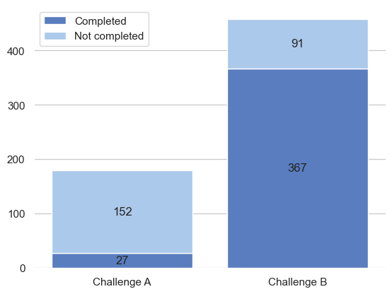
From this chart, visually at a glance, we can say that Challenge B has been completed more than Challenge A. Although they have different supporters registered on them so it’s not really obvious to compare if we use the completion rate ratio Challenge B in fact has a higher rate (80.13%) than Challenge A (15.08%) the difference is around 65% which is pretty huge.

From there raise a question or some of us may ask why Challenge B has more completion rate than A? It’s related to the maximum of total_actions needed to complete the challenge.

Total Actions

Using the total actions feature we can see how many actions the supporter have been take other than the maximum actions or completed the challenge.

data = dfa_start['Total Action'].value_counts().rename_axis('total actions').reset_index(name='counts')

Using the challenge_a_start dataset we can use value_counts to count the occurrences of unique values in this case the supporters with total actions of 1,2,3 etc.

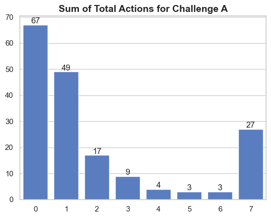
Using previous data we can plot the chart for Challenge A and we can apply the same process for Challenge B.

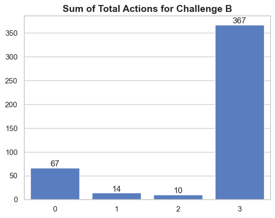
From total_actions we can see the majority of 67 supporters on Challenge A have taken 0 actions while the supporters on Challenge B have taken the maximum number of actions or completed the challenge. Interestingly enough good number of 49 supporters on Challenge A have taken 1 action but they didn’t finish the challenge.

Completed Actions Per Week

By processing the Total Time (day) feature we can see how much time is needed for the supporters to finish the challenge.

data = dfa_complete.copy()
data.loc[data['Total Time (Day)'] <= 7, 'Total Time (Day)'] = 1
data.loc[(data['Total Time (Day)'] > 7) & (data['Total Time (Day)'] <= 14), 'Total Time (Day)'] = 2
data.loc[(data['Total Time (Day)'] > 14) & (data['Total Time (Day)'] <= 21), 'Total Time (Day)'] = 3
data.loc[ data['Total Time (Day)'] > 21, 'Total Time (Day)'] = 4

Using the chalenge_a_completed dataset with the Total Time (day) feature, instead of using day format we process the data to be categorically using the binning technique to show the difference of completed challenges throughout the weeks.

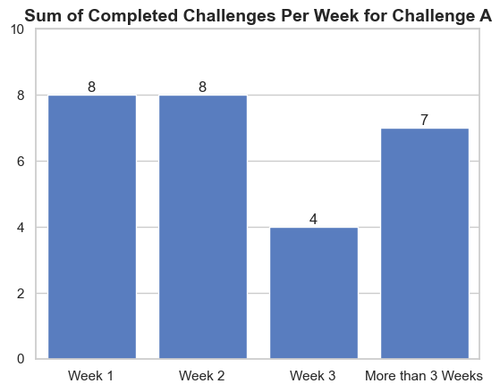
Plot the data and we got to see this chart for Challenge A. Do the same process for Challenge B.

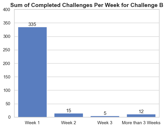
From here we can see that Challenge A differs from Challenge B in terms of how many supporters completed the challenge on a different week. Challenge A have been completed vary across different week while Challenge B have been completed on the first week.

Summary

• In general Challenge A has more actions than Challenge B And, It turns out that:
  • Challenge B has more completion rate than Challenge A
  • The majority of Challenge B has been completed in the first week compared to Challenge A which varies across different weeks

Key Insight

“Total Actions play a key role in gathering supporters”

The larger the actions will affect the amount of times of supporter finishes the challenge, it also affects the completion rate or whether the supporter will finish the challenge or not. It can also imply that,

“The amount of effort that the supporter needs to finish the challenge will affect the number of supporters”

Things like the complexity of the actions will also potentially affect the number of supporters

Recommendations

Based on the key findings if the goal is to gain supporters, It is recommended to:

• Use a lesser number of actions when creating a challenge.
• Don’t make actions that are too complicated.

Because it takes more effort for the supporter to finish the challenge, so simplicity is the key.

And that pretty much answers all of the project objectives the summarization of the project is also available in the form of Google Slides below: