Cyclistic Bike-Share Analysis
This is a Capstone Project for the Google Data Analytics Professional Certification.
Project Report

Learning Objective
- Going through the Ask, Prepare, Process, Analyze, and Share phases of the data analysis process
- Stating a business task clearly
- Importing data from a real dataset
- Documenting any data cleaning that you perform on the dataset
- Analyzing the data
- Creating data visualizations from analysis
- Summarizing key findings from analysis
- Documenting conclusions and recommendations
- Creating and publishing case study
Scenario
Junior data analyst working in the marketing analyst team at Cyclistic, a bike-share company in Chicago. The director of marketing and Cyclistic’s finance analysts believes the company’s future success depends on maximizing the number of annual memberships. Therefore, your team wants to understand how casual riders and annual members use Cyclistic bikes differently. From these insights, your team will design a new marketing strategy to convert casual riders into annual members. But first, Cyclistic executives must approve your recommendations, so they must be backed up with compelling data insights and professional data visualizations
About Cyclistic
![]()
In 2016, Cyclistic launched a successful bike-share offering. Since then, the program has grown to a fleet of 5,824 bicycles that are geotracked and locked into a network of 692 stations across Chicago. The bikes can be unlocked from one station and returned to any other station in the system anytime. Until now, Cyclistic’s marketing strategy relied on building general awareness and appealing to broad consumer segments. One approach that helped make these things possible was the flexibility of its pricing plans: single-ride passes, full-day passes, and annual memberships. Customers who purchase single-ride or full-day passes are referred to as casual riders. Customers who purchase annual memberships are Cyclistic members. Cyclistic’s finance analysts have concluded that annual members are much more profitable than casual riders. Although the pricing flexibility helps Cyclistic attract more customers, Moreno believes that maximizing the number of annual members will be key to future growth. Rather than creating a marketing campaign that targets all-new customers, Moreno believes there is a very good chance to convert casual riders into members. She notes that casual riders are already aware of the Cyclistic program and have chosen Cyclistic for their mobility needs. Moreno has set a clear goal: Design marketing strategies aimed at converting casual riders into annual members. In order to do that, however, the marketing analyst team needs to better understand how annual members and casual riders differ, why casual riders would buy a membership, and how digital media could affect their marketing tactics. Moreno and her team are interested in analyzing the Cyclistic historical bike trip data to identify trends.
Getting Started
I will be using the 6 phases of the analysis process (Ask, Prepare, Process, Analyse, Share and Act) to help guide my analysis, as it’s one of the most common use workflows for data analysts.
Phase 1: Ask
It’s important to understand the problem and any questions about case study early on so that you’re focused on your stakeholders’ needs.
Identify Business Task
Based on the scenario provided the topic of analytics is revolve around maximizing the number of annual memberships, however, to achieve this we need to have a better understanding of our market segment, how casual riders and annual members use Cyclistic bikes differently. there are several questions we could ask:
- How do annual members and casual riders use Cyclistic bikes differently?
- Why would casual riders buy Cyclistic annual memberships?
- How can Cyclistic use digital media to influence casual riders to become members?
Consider Key Stakeholders
Primary Stakeholder(s):
- Lily Moreno - The Director of Marketing
- Cyclistic Marketing Analytics Team
- Cyclistic Executive Team
Phase 2: Prepare
The prepare phase ensures that we have all of the data we need for our analysis and that we have credible and useful data.
Identify the data source
Dataset: Cyclistic’s historical trip data available here (Note: The datasets have a different name because Cyclistic is a fictional company. For the purposes of this case study, the datasets are appropriate and will enable us to answer the business questions. The data has been made available by Motivate International Inc. under this license.). This is public data that we can use to explore how different customer types are using Cyclistic bikes.
Determine the credibility of the data
For this task one common way to validate our data is by using ROCCC
- Reliability : Reliability means data can be trusted because it’s accurate, complete, and unbiased. There is no information provided about sample size and margin of error, so we’re not 100% sure about this.
- Originality : This data is collected directly from Cyclistic database (First-Party data) which is the original source
- Comprehensive : Comprehensive means data is not missing important information needed to answer business question, as stated in the previous section the datasets are appropriate and will enable us to answer the business questions. (For the purpose of this case study)
- Current : The recent data available that is complete for 12 months period came from 2019, which means it is currently outdated and may not represent the current trends in bike ride usage
- Cited : The data has been made available by Motivate International Inc under this license
NOTE: as you can see the current data doesn’t pass all the ROCCC checklist, as mentioned in the previous section this is still appropriate for the sake of simplicity of our case study we can go to the next section. However, checking the credibility of our data is important in real-world scenarios because bad data can skew our analysis result which can lead to a bad business decision.
Inspect our data
By inspecting it we can identify problems, and verify the integrity of our data. First of all, let’s load the required packages by using xfun package, it’s make sure that we have installed and load all the required packages defined in the vector
require(xfun)
## Loading required package: xfun

##
## Attaching package: 'xfun'

## The following objects are masked from 'package:base':
##
##     attr, isFALSE
packages <- c('tidyverse', # for data importing and wrangling
              'lubridate', # for date functions
              'ggplot2' # for visualization
              )
xfun::pkg_attach2(packages, message = FALSE)
Now let’s load our data, there are 4 data that is represented by different quarters from 2019 to 2020 (the most recent data)
q1_2020 <- read_csv("Divvy_Trips_2020_Q1.csv")
q2_2019 <- read_csv("Divvy_Trips_2019_Q2.csv")
q3_2019 <- read_csv("Divvy_Trips_2019_Q3.csv")
q4_2019 <- read_csv("Divvy_Trips_2019_Q4.csv")
First of all let’s take a look at the data, understand how they look using colnames()
colnames(q1_2020)
##  [1] "ride_id"            "rideable_type"      "started_at"
##  [4] "ended_at"           "start_station_name" "start_station_id"
##  [7] "end_station_name"   "end_station_id"     "start_lat"
## [10] "start_lng"          "end_lat"            "end_lng"
## [13] "member_casual"
colnames(q2_2019)
##  [1] "01 - Rental Details Rental ID"
##  [2] "01 - Rental Details Local Start Time"
##  [3] "01 - Rental Details Local End Time"
##  [4] "01 - Rental Details Bike ID"
##  [5] "01 - Rental Details Duration In Seconds Uncapped"
##  [6] "03 - Rental Start Station ID"
##  [7] "03 - Rental Start Station Name"
##  [8] "02 - Rental End Station ID"
##  [9] "02 - Rental End Station Name"
## [10] "User Type"
## [11] "Member Gender"
## [12] "05 - Member Details Member Birthday Year"
colnames(q3_2019)
##  [1] "trip_id"           "start_time"        "end_time"
##  [4] "bikeid"            "tripduration"      "from_station_id"
##  [7] "from_station_name" "to_station_id"     "to_station_name"
## [10] "usertype"          "gender"            "birthyear"
colnames(q4_2019)
##  [1] "trip_id"           "start_time"        "end_time"
##  [4] "bikeid"            "tripduration"      "from_station_id"
##  [7] "from_station_name" "to_station_id"     "to_station_name"
## [10] "usertype"          "gender"            "birthyear"
after running the above code we will notice that the data doesn’t have the same column, so we need to rename it, to make the column name consistent, we will use the q1_2020 data as our naming reference.
(q4_2019 <- rename(q4_2019
                   ,ride_id = trip_id
                   ,rideable_type = bikeid
                   ,started_at = start_time
                   ,ended_at = end_time
                   ,start_station_name = from_station_name
                   ,start_station_id = from_station_id
                   ,end_station_name = to_station_name
                   ,end_station_id = to_station_id
                   ,member_casual = usertype))
(q3_2019 <- rename(q3_2019
                   ,ride_id = trip_id
                   ,rideable_type = bikeid
                   ,started_at = start_time
                   ,ended_at = end_time
                   ,start_station_name = from_station_name
                   ,start_station_id = from_station_id
                   ,end_station_name = to_station_name
                   ,end_station_id = to_station_id
                   ,member_casual = usertype))
(q2_2019 <- rename(q2_2019
                   ,ride_id = "01 - Rental Details Rental ID"
                   ,rideable_type = "01 - Rental Details Bike ID"
                   ,started_at = "01 - Rental Details Local Start Time"
                   ,ended_at = "01 - Rental Details Local End Time"
                   ,start_station_name = "03 - Rental Start Station Name"
                   ,start_station_id = "03 - Rental Start Station ID"
                   ,end_station_name = "02 - Rental End Station Name"
                   ,end_station_id = "02 - Rental End Station ID"
                   ,member_casual = "User Type"))
# Inspect the dataframes and look for incongruencies
str(q1_2020)
## spec_tbl_df [426,887 × 13] (S3: spec_tbl_df/tbl_df/tbl/data.frame)
##  $ ride_id           : chr [1:426887] "EACB19130B0CDA4A" "8FED874C809DC021" "789F3C21E472CA96" "C9A388DAC6ABF313" ...
##  $ rideable_type     : chr [1:426887] "docked_bike" "docked_bike" "docked_bike" "docked_bike" ...
##  $ started_at        : POSIXct[1:426887], format: "2020-01-21 20:06:59" "2020-01-30 14:22:39" ...
##  $ ended_at          : POSIXct[1:426887], format: "2020-01-21 20:14:30" "2020-01-30 14:26:22" ...
##  $ start_station_name: chr [1:426887] "Western Ave & Leland Ave" "Clark St & Montrose Ave" "Broadway & Belmont Ave" "Clark St & Randolph St" ...
##  $ start_station_id  : num [1:426887] 239 234 296 51 66 212 96 96 212 38 ...
##  $ end_station_name  : chr [1:426887] "Clark St & Leland Ave" "Southport Ave & Irving Park Rd" "Wilton Ave & Belmont Ave" "Fairbanks Ct & Grand Ave" ...
##  $ end_station_id    : num [1:426887] 326 318 117 24 212 96 212 212 96 100 ...
##  $ start_lat         : num [1:426887] 42 42 41.9 41.9 41.9 ...
##  $ start_lng         : num [1:426887] -87.7 -87.7 -87.6 -87.6 -87.6 ...
##  $ end_lat           : num [1:426887] 42 42 41.9 41.9 41.9 ...
##  $ end_lng           : num [1:426887] -87.7 -87.7 -87.7 -87.6 -87.6 ...
##  $ member_casual     : chr [1:426887] "member" "member" "member" "member" ...
##  - attr(*, "spec")=
##   .. cols(
##   ..   ride_id = col_character(),
##   ..   rideable_type = col_character(),
##   ..   started_at = col_datetime(format = ""),
##   ..   ended_at = col_datetime(format = ""),
##   ..   start_station_name = col_character(),
##   ..   start_station_id = col_double(),
##   ..   end_station_name = col_character(),
##   ..   end_station_id = col_double(),
##   ..   start_lat = col_double(),
##   ..   start_lng = col_double(),
##   ..   end_lat = col_double(),
##   ..   end_lng = col_double(),
##   ..   member_casual = col_character()
##   .. )
##  - attr(*, "problems")=<externalptr>
str(q4_2019)
## spec_tbl_df [704,054 × 12] (S3: spec_tbl_df/tbl_df/tbl/data.frame)
##  $ ride_id           : num [1:704054] 25223640 25223641 25223642 25223643 25223644 ...
##  $ started_at        : POSIXct[1:704054], format: "2019-10-01 00:01:39" "2019-10-01 00:02:16" ...
##  $ ended_at          : POSIXct[1:704054], format: "2019-10-01 00:17:20" "2019-10-01 00:06:34" ...
##  $ rideable_type     : num [1:704054] 2215 6328 3003 3275 5294 ...
##  $ tripduration      : num [1:704054] 940 258 850 2350 1867 ...
##  $ start_station_id  : num [1:704054] 20 19 84 313 210 156 84 156 156 336 ...
##  $ start_station_name: chr [1:704054] "Sheffield Ave & Kingsbury St" "Throop (Loomis) St & Taylor St" "Milwaukee Ave & Grand Ave" "Lakeview Ave & Fullerton Pkwy" ...
##  $ end_station_id    : num [1:704054] 309 241 199 290 382 226 142 463 463 336 ...
##  $ end_station_name  : chr [1:704054] "Leavitt St & Armitage Ave" "Morgan St & Polk St" "Wabash Ave & Grand Ave" "Kedzie Ave & Palmer Ct" ...
##  $ member_casual     : chr [1:704054] "Subscriber" "Subscriber" "Subscriber" "Subscriber" ...
##  $ gender            : chr [1:704054] "Male" "Male" "Female" "Male" ...
##  $ birthyear         : num [1:704054] 1987 1998 1991 1990 1987 ...
##  - attr(*, "spec")=
##   .. cols(
##   ..   trip_id = col_double(),
##   ..   start_time = col_datetime(format = ""),
##   ..   end_time = col_datetime(format = ""),
##   ..   bikeid = col_double(),
##   ..   tripduration = col_number(),
##   ..   from_station_id = col_double(),
##   ..   from_station_name = col_character(),
##   ..   to_station_id = col_double(),
##   ..   to_station_name = col_character(),
##   ..   usertype = col_character(),
##   ..   gender = col_character(),
##   ..   birthyear = col_double()
##   .. )
##  - attr(*, "problems")=<externalptr>
str(q3_2019)
## spec_tbl_df [1,640,718 × 12] (S3: spec_tbl_df/tbl_df/tbl/data.frame)
##  $ ride_id           : num [1:1640718] 23479388 23479389 23479390 23479391 23479392 ...
##  $ started_at        : POSIXct[1:1640718], format: "2019-07-01 00:00:27" "2019-07-01 00:01:16" ...
##  $ ended_at          : POSIXct[1:1640718], format: "2019-07-01 00:20:41" "2019-07-01 00:18:44" ...
##  $ rideable_type     : num [1:1640718] 3591 5353 6180 5540 6014 ...
##  $ tripduration      : num [1:1640718] 1214 1048 1554 1503 1213 ...
##  $ start_station_id  : num [1:1640718] 117 381 313 313 168 300 168 313 43 43 ...
##  $ start_station_name: chr [1:1640718] "Wilton Ave & Belmont Ave" "Western Ave & Monroe St" "Lakeview Ave & Fullerton Pkwy" "Lakeview Ave & Fullerton Pkwy" ...
##  $ end_station_id    : num [1:1640718] 497 203 144 144 62 232 62 144 195 195 ...
##  $ end_station_name  : chr [1:1640718] "Kimball Ave & Belmont Ave" "Western Ave & 21st St" "Larrabee St & Webster Ave" "Larrabee St & Webster Ave" ...
##  $ member_casual     : chr [1:1640718] "Subscriber" "Customer" "Customer" "Customer" ...
##  $ gender            : chr [1:1640718] "Male" NA NA NA ...
##  $ birthyear         : num [1:1640718] 1992 NA NA NA NA ...
##  - attr(*, "spec")=
##   .. cols(
##   ..   trip_id = col_double(),
##   ..   start_time = col_datetime(format = ""),
##   ..   end_time = col_datetime(format = ""),
##   ..   bikeid = col_double(),
##   ..   tripduration = col_number(),
##   ..   from_station_id = col_double(),
##   ..   from_station_name = col_character(),
##   ..   to_station_id = col_double(),
##   ..   to_station_name = col_character(),
##   ..   usertype = col_character(),
##   ..   gender = col_character(),
##   ..   birthyear = col_double()
##   .. )
##  - attr(*, "problems")=<externalptr>
str(q2_2019)
## spec_tbl_df [1,108,163 × 12] (S3: spec_tbl_df/tbl_df/tbl/data.frame)
##  $ ride_id                                         : num [1:1108163] 22178529 22178530 22178531 22178532 22178533 ...
##  $ started_at                                      : POSIXct[1:1108163], format: "2019-04-01 00:02:22" "2019-04-01 00:03:02" ...
##  $ ended_at                                        : POSIXct[1:1108163], format: "2019-04-01 00:09:48" "2019-04-01 00:20:30" ...
##  $ rideable_type                                   : num [1:1108163] 6251 6226 5649 4151 3270 ...
##  $ 01 - Rental Details Duration In Seconds Uncapped: num [1:1108163] 446 1048 252 357 1007 ...
##  $ start_station_id                                : num [1:1108163] 81 317 283 26 202 420 503 260 211 211 ...
##  $ start_station_name                              : chr [1:1108163] "Daley Center Plaza" "Wood St & Taylor St" "LaSalle St & Jackson Blvd" "McClurg Ct & Illinois St" ...
##  $ end_station_id                                  : num [1:1108163] 56 59 174 133 129 426 500 499 211 211 ...
##  $ end_station_name                                : chr [1:1108163] "Desplaines St & Kinzie St" "Wabash Ave & Roosevelt Rd" "Canal St & Madison St" "Kingsbury St & Kinzie St" ...
##  $ member_casual                                   : chr [1:1108163] "Subscriber" "Subscriber" "Subscriber" "Subscriber" ...
##  $ Member Gender                                   : chr [1:1108163] "Male" "Female" "Male" "Male" ...
##  $ 05 - Member Details Member Birthday Year        : num [1:1108163] 1975 1984 1990 1993 1992 ...
##  - attr(*, "spec")=
##   .. cols(
##   ..   `01 - Rental Details Rental ID` = col_double(),
##   ..   `01 - Rental Details Local Start Time` = col_datetime(format = ""),
##   ..   `01 - Rental Details Local End Time` = col_datetime(format = ""),
##   ..   `01 - Rental Details Bike ID` = col_double(),
##   ..   `01 - Rental Details Duration In Seconds Uncapped` = col_number(),
##   ..   `03 - Rental Start Station ID` = col_double(),
##   ..   `03 - Rental Start Station Name` = col_character(),
##   ..   `02 - Rental End Station ID` = col_double(),
##   ..   `02 - Rental End Station Name` = col_character(),
##   ..   `User Type` = col_character(),
##   ..   `Member Gender` = col_character(),
##   ..   `05 - Member Details Member Birthday Year` = col_double()
##   .. )
##  - attr(*, "problems")=<externalptr>
if you see the ride_id and rideable_type column in q1_2020 doesn’t have the same data type with the others, so we need to convert it, because we want to merge the data later on, and it’s not possible if same column have different data type
q4_2019 <-  mutate(q4_2019, ride_id = as.character(ride_id)
                   ,rideable_type = as.character(rideable_type))
q3_2019 <-  mutate(q3_2019, ride_id = as.character(ride_id)
                   ,rideable_type = as.character(rideable_type))
q2_2019 <-  mutate(q2_2019, ride_id = as.character(ride_id)
                   ,rideable_type = as.character(rideable_type))
after we make sure, the specific column has the same data type, we can start merge into a single variable called all_trips
all_trips <- bind_rows(q2_2019, q3_2019, q4_2019, q1_2020)
Remove lat, long, birthyear, and gender fields as this data was dropped beginning in 2020
all_trips <- all_trips %>%
  select(-c(start_lat, start_lng, end_lat, end_lng, birthyear, gender, "01 - Rental Details Duration In Seconds Uncapped", "05 - Member Details Member Birthday Year", "Member Gender", "tripduration"))
Phase 3: Process
Now that we know our data is credible and relevant to our problem, we’ll need to clean it so that our analysis will be error-free. first, we’re going to take a look at our merged data.
colnames(all_trips) #List of column names
## [1] "ride_id"            "started_at"         "ended_at"
## [4] "rideable_type"      "start_station_id"   "start_station_name"
## [7] "end_station_id"     "end_station_name"   "member_casual"
nrow(all_trips) #How many rows are in data frame?
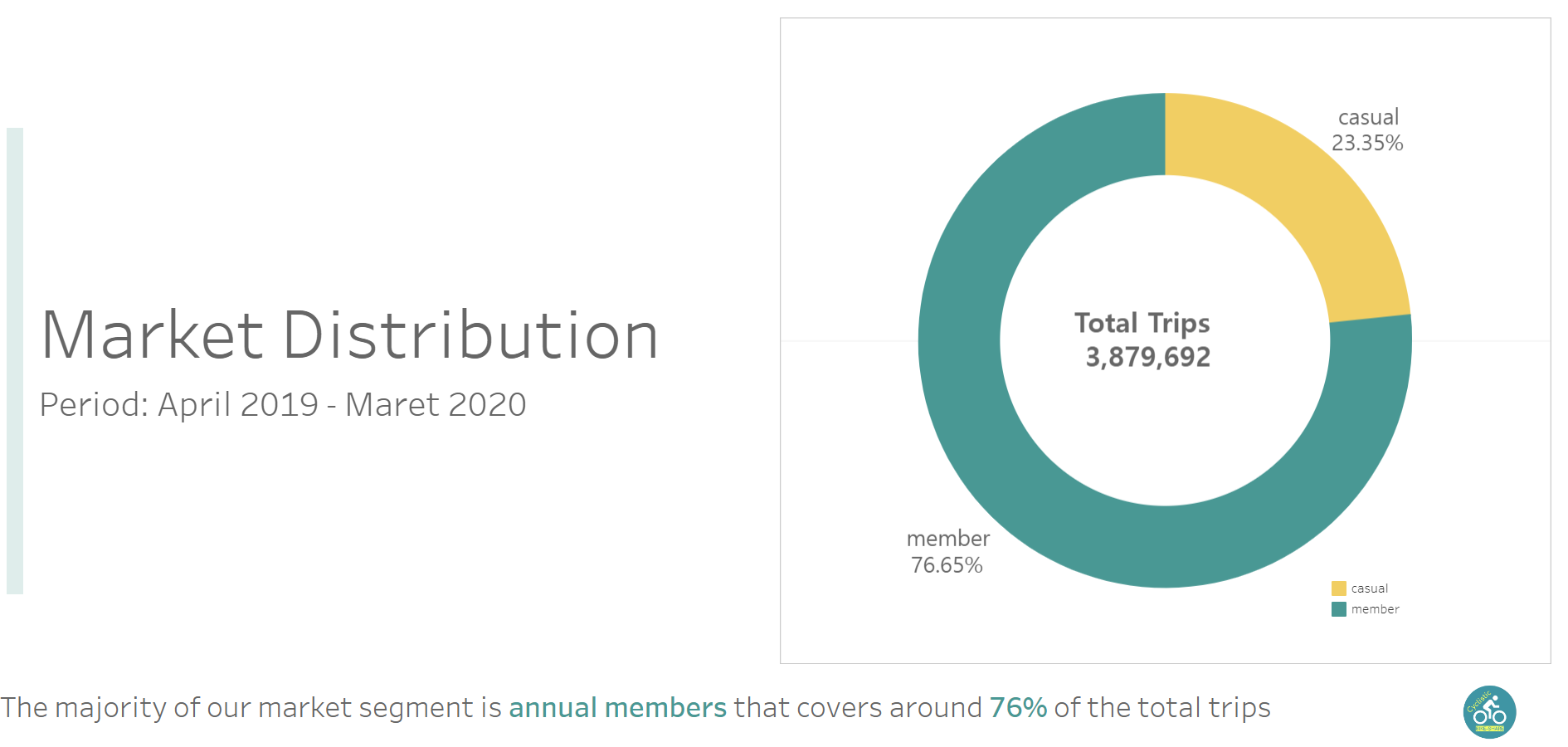
## [1] 3879822
dim(all_trips) #Dimensions of the data frame?
## [1] 3879822 9
head(all_trips) #See the first 6 rows of data frame. Also tail(all_trips)
## # A tibble: 6 × 9
##   ride_id started_at          ended_at            rideable_type start_station_id
##   <chr>   <dttm>              <dttm>              <chr>                    <dbl>
## 1 221785… 2019-04-01 00:02:22 2019-04-01 00:09:48 6251                        81
## 2 221785… 2019-04-01 00:03:02 2019-04-01 00:20:30 6226                       317
## 3 221785… 2019-04-01 00:11:07 2019-04-01 00:15:19 5649                       283
## 4 221785… 2019-04-01 00:13:01 2019-04-01 00:18:58 4151                        26
## 5 221785… 2019-04-01 00:19:26 2019-04-01 00:36:13 3270                       202
## 6 221785… 2019-04-01 00:19:39 2019-04-01 00:23:56 3123                       420
## # … with 4 more variables: start_station_name <chr>, end_station_id <dbl>,
## #   end_station_name <chr>, member_casual <chr>
str(all_trips) #See list of columns and data types (numeric, character, etc)
## tibble [3,879,822 × 9] (S3: tbl_df/tbl/data.frame)
##  $ ride_id           : chr [1:3879822] "22178529" "22178530" "22178531" "22178532" ...
##  $ started_at        : POSIXct[1:3879822], format: "2019-04-01 00:02:22" "2019-04-01 00:03:02" ...
##  $ ended_at          : POSIXct[1:3879822], format: "2019-04-01 00:09:48" "2019-04-01 00:20:30" ...
##  $ rideable_type     : chr [1:3879822] "6251" "6226" "5649" "4151" ...
##  $ start_station_id  : num [1:3879822] 81 317 283 26 202 420 503 260 211 211 ...
##  $ start_station_name: chr [1:3879822] "Daley Center Plaza" "Wood St & Taylor St" "LaSalle St & Jackson Blvd" "McClurg Ct & Illinois St" ...
##  $ end_station_id    : num [1:3879822] 56 59 174 133 129 426 500 499 211 211 ...
##  $ end_station_name  : chr [1:3879822] "Desplaines St & Kinzie St" "Wabash Ave & Roosevelt Rd" "Canal St & Madison St" "Kingsbury St & Kinzie St" ...
##  $ member_casual     : chr [1:3879822] "Subscriber" "Subscriber" "Subscriber" "Subscriber" ...
summary(all_trips) #Statistical summary of data. Mainly for numerics
##    ride_id            started_at
##  Length:3879822     Min.   :2019-04-01 00:02:22.00
##  Class :character   1st Qu.:2019-06-23 07:49:09.25
##  Mode  :character   Median :2019-08-14 17:43:38.00
##                     Mean   :2019-08-26 00:49:59.38
##                     3rd Qu.:2019-10-12 12:10:21.00
##                     Max.   :2020-03-31 23:51:34.00
##
##     ended_at                      rideable_type      start_station_id
##  Min.   :2019-04-01 00:09:48.00   Length:3879822     Min.   :  1.0
##  1st Qu.:2019-06-23 08:20:27.75   Class :character   1st Qu.: 77.0
##  Median :2019-08-14 18:02:04.00   Mode  :character   Median :174.0
##  Mean   :2019-08-26 01:14:37.06                      Mean   :202.9
##  3rd Qu.:2019-10-12 12:36:16.75                      3rd Qu.:291.0
##  Max.   :2020-05-19 20:10:34.00                      Max.   :675.0
##
##  start_station_name end_station_id  end_station_name   member_casual
##  Length:3879822     Min.   :  1.0   Length:3879822     Length:3879822
##  Class :character   1st Qu.: 77.0   Class :character   Class :character
##  Mode  :character   Median :174.0   Mode  :character   Mode  :character
##                     Mean   :203.8
##                     3rd Qu.:291.0
##                     Max.   :675.0
##                     NA's   :1
If you notice, there are few problems we will need to fix:
- In the “member_casual” column, there are two names for members (“member” and “Subscriber”) and two names for casual riders (“Customer” and “casual”). We will need to consolidate that from four to two labels.
- The data can only be aggregated at the ride-level, which is too granular. We will want to add some additional columns of data – such as day, month, year – that provide additional opportunities to aggregate the data.
- We will want to add a calculated field for length of ride since the 2020Q1 data did not have the “tripduration” column. We will add “ride_length” to the entire dataframe for consistency.
- There are some rides where tripduration shows up as negative, including several hundred rides where Divvy took bikes out of circulation for Quality Control reasons. We will want to delete these rides.
Reassign to the desired values (we will go with the current 2020 labels)
all_trips <-  all_trips %>%
  mutate(member_casual = recode(member_casual
                           ,"Subscriber" = "member"
                           ,"Customer" = "casual"))
Check to make sure the proper number of observations were reassigned
table(all_trips$member_casual)
##
##  casual  member
##  905954 2973868
Add columns that list the date, month, day, and year of each ride, this will allow us to aggregate ride data for each month, day, or year
all_trips$date <- as.Date(all_trips$started_at) #The default format is yyyy-mm-dd
all_trips$month <- format(as.Date(all_trips$date), "%m")
all_trips$day <- format(as.Date(all_trips$date), "%d")
all_trips$year <- format(as.Date(all_trips$date), "%Y")
all_trips$day_of_week <- format(as.Date(all_trips$date), "%A")
Add a “ride_length” calculation to all_trips (in seconds)
all_trips$ride_length <- difftime(all_trips$ended_at,all_trips$started_at)
str(all_trips)
## tibble [3,879,822 × 15] (S3: tbl_df/tbl/data.frame)
##  $ ride_id           : chr [1:3879822] "22178529" "22178530" "22178531" "22178532" ...
##  $ started_at        : POSIXct[1:3879822], format: "2019-04-01 00:02:22" "2019-04-01 00:03:02" ...
##  $ ended_at          : POSIXct[1:3879822], format: "2019-04-01 00:09:48" "2019-04-01 00:20:30" ...
##  $ rideable_type     : chr [1:3879822] "6251" "6226" "5649" "4151" ...
##  $ start_station_id  : num [1:3879822] 81 317 283 26 202 420 503 260 211 211 ...
##  $ start_station_name: chr [1:3879822] "Daley Center Plaza" "Wood St & Taylor St" "LaSalle St & Jackson Blvd" "McClurg Ct & Illinois St" ...
##  $ end_station_id    : num [1:3879822] 56 59 174 133 129 426 500 499 211 211 ...
##  $ end_station_name  : chr [1:3879822] "Desplaines St & Kinzie St" "Wabash Ave & Roosevelt Rd" "Canal St & Madison St" "Kingsbury St & Kinzie St" ...
##  $ member_casual     : chr [1:3879822] "member" "member" "member" "member" ...
##  $ date              : Date[1:3879822], format: "2019-04-01" "2019-04-01" ...
##  $ month             : chr [1:3879822] "04" "04" "04" "04" ...
##  $ day               : chr [1:3879822] "01" "01" "01" "01" ...
##  $ year              : chr [1:3879822] "2019" "2019" "2019" "2019" ...
##  $ day_of_week       : chr [1:3879822] "Monday" "Monday" "Monday" "Monday" ...
##  $ ride_length       : 'difftime' num [1:3879822] 446 1048 252 357 ...
##   ..- attr(*, "units")= chr "secs"
Convert “ride_length” from Factor to numeric so we can run calculations on the data
all_trips$ride_length <- as.numeric(as.character(all_trips$ride_length))
is.numeric(all_trips$ride_length)
## [1] TRUE
The dataframe includes a few hundred negative entries in ride_length, and it’s stated in the study case that it’s fine to drop it.
all_trips_v2 <- all_trips[!(all_trips$ride_length<0),]
Phase 4: Analyze
Now we’ll really put our data to work to uncover new insights and discover potential solutions to our problem! conduct simple analysis to help answer the key question: “In what ways do members and casual riders use Divvy bikes differently?”
Conduct Descriptive Analysis
Let’s perform descriptive analysis on ride_length with summary() function
summary(all_trips_v2$ride_length)
##    Min. 1st Qu.  Median    Mean 3rd Qu.    Max.
##       0     411     711    1478    1288 9387024
Compare members and casual users
aggregate(all_trips_v2$ride_length ~ all_trips_v2$member_casual, FUN = mean)
##   all_trips_v2$member_casual all_trips_v2$ride_length
## 1                     casual                3538.4516
## 2                     member                 850.0659
aggregate(all_trips_v2$ride_length ~ all_trips_v2$member_casual, FUN = median)
##   all_trips_v2$member_casual all_trips_v2$ride_length
## 1                     casual                     1540
## 2                     member                      589
aggregate(all_trips_v2$ride_length ~ all_trips_v2$member_casual, FUN = max)
##   all_trips_v2$member_casual all_trips_v2$ride_length
## 1                     casual                  9387024
## 2                     member                  9056634
aggregate(all_trips_v2$ride_length ~ all_trips_v2$member_casual, FUN = min)
##   all_trips_v2$member_casual all_trips_v2$ride_length
## 1                     casual                        0
## 2                     member                        1
See the average ride time by each day for members vs casual users
aggregate(all_trips_v2$ride_length ~ all_trips_v2$member_casual + all_trips_v2$day_of_week, FUN = mean)
##    all_trips_v2$member_casual all_trips_v2$day_of_week all_trips_v2$ride_length
## 1                      casual                   Friday                3758.2210
## 2                      member                   Friday                 824.5305
## 3                      casual                   Monday                3335.6446
## 4                      member                   Monday                 842.5726
## 5                      casual                 Saturday                3331.9138
## 6                      member                 Saturday                 968.9337
## 7                      casual                   Sunday                3581.4054
## 8                      member                   Sunday                 919.9746
## 9                      casual                 Thursday                3660.2933
## 10                     member                 Thursday                 823.9278
## 11                     casual                  Tuesday                3569.7986
## 12                     member                  Tuesday                 826.1427
## 13                     casual                Wednesday                3691.0203
## 14                     member                Wednesday                 823.9980
Notice that the days of the week are out of order. Let’s fix that
all_trips_v2$day_of_week <- ordered(all_trips_v2$day_of_week, levels=c("Sunday", "Monday", "Tuesday", "Wednesday", "Thursday", "Friday", "Saturday"))
Now, let’s run the average ride time by each day for members vs casual users
aggregate(all_trips_v2$ride_length ~ all_trips_v2$member_casual + all_trips_v2$day_of_week, FUN = mean)
##    all_trips_v2$member_casual all_trips_v2$day_of_week all_trips_v2$ride_length
## 1                      casual                   Sunday                3581.4054
## 2                      member                   Sunday                 919.9746
## 3                      casual                   Monday                3335.6446
## 4                      member                   Monday                 842.5726
## 5                      casual                  Tuesday                3569.7986
## 6                      member                  Tuesday                 826.1427
## 7                      casual                Wednesday                3691.0203
## 8                      member                Wednesday                 823.9980
## 9                      casual                 Thursday                3660.2933
## 10                     member                 Thursday                 823.9278
## 11                     casual                   Friday                3758.2210
## 12                     member                   Friday                 824.5305
## 13                     casual                 Saturday                3331.9138
## 14                     member                 Saturday                 968.9337
Analyze ridership data by type and weekday
all_trips_v2 %>%
  mutate(weekday = wday(started_at, label = TRUE)) %>%  #creates weekday field using wday()
  group_by(member_casual, weekday) %>%  #groups by usertype and weekday
  summarise(number_of_rides = n()                           #calculates the number of rides and average duration
  ,average_duration = mean(ride_length)) %>%        # calculates the average duration
  arrange(member_casual, weekday)
## `summarise()` has grouped output by 'member_casual'. You can override using the
## `.groups` argument.

## # A tibble: 14 × 4
## # Groups:   member_casual [2]
##    member_casual weekday number_of_rides average_duration
##    <chr>         <ord>             <int>            <dbl>
##  1 casual        Sun              181293            3581.
##  2 casual        Mon              104432            3336.
##  3 casual        Tue               91184            3570.
##  4 casual        Wed               93150            3691.
##  5 casual        Thu              103316            3660.
##  6 casual        Fri              122913            3758.
##  7 casual        Sat              209543            3332.
##  8 member        Sun              267965             920.
##  9 member        Mon              472196             843.
## 10 member        Tue              508445             826.
## 11 member        Wed              500330             824.
## 12 member        Thu              484177             824.
## 13 member        Fri              452790             825.
## 14 member        Sat              287958             969.
Let’s visualize the number of rides by rider type
all_trips_v2 %>%
  mutate(weekday = wday(started_at, label = TRUE)) %>%
  group_by(member_casual, weekday) %>%
  summarise(number_of_rides = n()
            ,average_duration = mean(ride_length)) %>%
  arrange(member_casual, weekday)  %>%
  ggplot(aes(x = weekday, y = number_of_rides, fill = member_casual)) +
  geom_col(position = "dodge")
## `summarise()` has grouped output by 'member_casual'. You can override using the
## `.groups` argument.
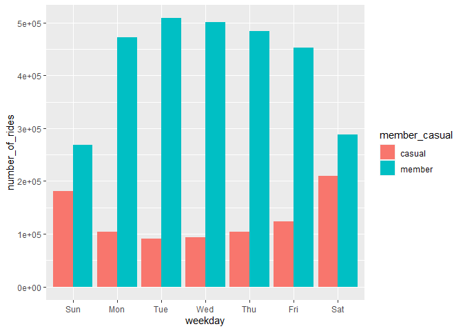
Based on this visualization we can see that annual_member have the highest average number of rides for the entire week, this might be due to cost efficiency that is offered for the annual member compared to casual member refer to this:
“Consumers can buy access to Divvy bikes using these options: (1) Single-ride passes for $3 per 30-minute trip; (2) Full-day passes for $15 per day for unlimited three-hour rides in a 24-hour period; and (3) Annual memberships for $99 per year for unlimited 45-minute rides. Small charges (15 cents per minute) are incurred when single rides exceed the maximum time allowance to dissuade consumers from checking out bikes and not returning them on time.” source: artscience
I also see negative correlation that is shared between casual and annual members, if we take a look at the chart above you can see that the number of rides for the annual membership is the highest on the weekend day and the lowest on the workday but it’s the opposite for the casual member, this might indicate that:
- major portion of annual members are using cyclictic for going to work (a trend on a workday), which might be a big factor why people use annual membership than the casual, in term of the cost it’s more efficient in a daily basis.
- major portion of casual members are using cyclistic for recreational purpose (a trend on weekend)
Let’s take a look at different perspective, by creating chart for average use duration
all_trips_v2 %>%
  mutate(weekday = wday(started_at, label = TRUE)) %>%
  group_by(member_casual, weekday) %>%
  summarise(number_of_rides = n()
            ,average_duration = mean(ride_length)) %>%
  arrange(member_casual, weekday)  %>%
  ggplot(aes(x = weekday, y = average_duration, fill = member_casual)) +
  geom_col(position = "dodge")
## `summarise()` has grouped output by 'member_casual'. You can override using the
## `.groups` argument.
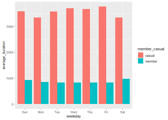
Based on this chart we can see that casual members have the highest average duration more than double of annual members, this might indicate that people want to maximize their bike usage based on what they paid, referring to the previous section casual members are the persons who use single ride passes for $3 per 30-minute trip and Full-day passes for $15 per day for unlimited three-hour rides in a 24-hour period and people who have annual membership tend to use in less duration considering they had access for the entire year and they only pay more if they use it more than 45 minutes.
But here’s the interesting one, again, the annual members shows the highest trend on the weekend and the lowest on the workday, based on the previous takeaways this might confirm that because the majority of people who had annual membership are using Cyclistic for work, they only using it for traveling between places, but in the weekdays they have much time outside desk, therefore the average duration is increased on weekday.
So after visualizing our data we can summarize that:
- Most of annual members use Cyclistic for work, while casual riders may use it for recreational purpose
- Because most of annual members use Cyclistic for work, it’s much more cost efficient to have annual membership because they use Cyclistic in a daily basis
And that’s pretty much answer first two question of our stakeholders
-
How do annual members and casual riders use Cyclistic bikes differently?
-
Why would casual riders buy Cyclistic annual memberships?
We can also extract our data for further more analysis using tableau.
By using Tableau I could visualize the data, analyzing it, while also generating a report using some of the features. Link