ID/X Loan Prediction

Task Background

As the final project of my contract period as an intern Data Scientist at ID/X Partners, this time I got involved in a project from a lending company and collaborate with various other departments on this project to provide technology solutions for the company. I got asked to build a model that can predict credit risk using a dataset provided by the company which consists of data on loans received and rejected. Besides that, I also need to prepare visual media to present solutions to clients. I need to make sure the visual media I create is clear, easy to read, and communicative. I can work on this end-to-end solution in the Programming Language of my choice while still referring to the Data Science framework/methodology.

The Objectives

Based on the task background the objectives of the project are:

• Building credit risk models
• Creating visual media as a form of Powerpoint presentation

Import Libraries

First of all, let’s start by importing all the necessary libraries. Libraries used in this project serve two different purposes some of them are for Data Exploration and Data Processing, and the others are for Modeling.

# Data Preprocessing
import imblearn
from imblearn.under_sampling import RandomUnderSampler
from imblearn.pipeline import Pipeline
from imblearn.over_sampling import SMOTE

from sklearn.preprocessing import RobustScaler

from collections import Counter
import category_encoders as ce

import pandas as pd
import numpy as np

import matplotlib.pyplot as plt
import seaborn as sns

# Modeling
import tensorflow as tf
from tensorflow.keras.models import Sequential
from tensorflow.keras.layers import Dense
from tensorflow.keras.activations import relu
from tensorflow.keras.losses import binary_crossentropy
from tensorflow.keras.optimizers import Adam

from sklearn import metrics
from sklearn.metrics import (accuracy_score, f1_score,average_precision_score, confusion_matrix,
                             average_precision_score, precision_score, recall_score, roc_auc_score, classification_report, roc_curve,auc, ConfusionMatrixDisplay )
from sklearn.ensemble import RandomForestClassifier
from sklearn.linear_model import LogisticRegression
from sklearn.model_selection import train_test_split

import xgboost as xgb

from pickle import dump

Data Understanding

The dataset used in this project is client loan data from 2007 to 2014 which has 73 features and consists of data on loans received and rejected. More information about the dataset can be accessed here: Data Dictionary

df = pd.read_csv("loan_data_2007_2014.csv", index_col=['id'])
df.head()

Using the above code we get to see a glimpse of the first five rows of the dataset.

id	member_id	loan_amnt	funded_amnt	funded_amnt_inv	term	int_rate	installment	grade	sub_grade
1077501	1296599	5000	5000	4975.0	36 months	10.65	162.87	B	B2
1077430	1314167	2500	2500	2500.0	60 months	15.27	59.83	C	C4
1077175	1313524	2400	2400	2400.0	36 months	15.96	84.33	C	C5
1076863	1277178	10000	10000	10000.0	36 months	13.49	339.31	C	C1
1075358	1311748	3000	3000	3000.0	60 months	12.69	67.79	B	B5

5 rows × 74 columns

Although there are so many features involved we get to see some of the important features like:

• grade: Usually represented by letters or alphanumeric symbols, and they may vary slightly depending on the specific lender or credit agency. Generally, the higher the loan grade, the lower the risk associated with the borrower, and therefore, the more favorable the terms of the loan (lower interest rates and fees) may be. A common loan grading system might look something like this:
  • Grade A: Very low risk, excellent creditworthiness.
  • Grade B: Low risk, very good creditworthiness.
  • Grade C: Moderate risk, good creditworthiness.
  • Grade D: Higher risk, fair creditworthiness.
  • Grade E: High risk, below-average creditworthiness.

  Lenders determine the loan grade by considering various factors such as the borrower’s credit score, credit history, income, debt-to-income ratio, employment stability, and other relevant financial information. It’s essential for borrowers to understand their loan grade as it directly impacts their ability to obtain a loan and the cost of borrowing. Lower loan grades may result in higher interest rates or even loan denials due to increased risk.

These features are important later since the dataset doesn’t have the target feature that corresponds to the loan application being accepted or rejected.

df.columns

Now, let’s see the whole features in the dataset. It can be achieved using the above code.

Index(['member_id', 'loan_amnt', 'funded_amnt', 'funded_amnt_inv', 'term',
       'int_rate', 'installment', 'grade', 'sub_grade', 'emp_title',
       'emp_length', 'home_ownership', 'annual_inc', 'verification_status',
       'issue_d', 'loan_status', 'pymnt_plan', 'url', 'desc', 'purpose',
       'title', 'zip_code', 'addr_state', 'dti', 'delinq_2yrs',
       'earliest_cr_line', 'inq_last_6mths', 'mths_since_last_delinq',
       'mths_since_last_record', 'open_acc', 'pub_rec', 'revol_bal',
       'revol_util', 'total_acc', 'initial_list_status', 'out_prncp',
       'out_prncp_inv', 'total_pymnt', 'total_pymnt_inv', 'total_rec_prncp',
       'total_rec_int', 'total_rec_late_fee', 'recoveries',
       'collection_recovery_fee', 'last_pymnt_d', 'last_pymnt_amnt',
       'next_pymnt_d', 'last_credit_pull_d', 'collections_12_mths_ex_med',
       'mths_since_last_major_derog', 'policy_code', 'application_type',
       'annual_inc_joint', 'dti_joint', 'verification_status_joint',
       'acc_now_delinq', 'tot_coll_amt', 'tot_cur_bal', 'open_acc_6m',
       'open_il_6m', 'open_il_12m', 'open_il_24m', 'mths_since_rcnt_il',
       'total_bal_il', 'il_util', 'open_rv_12m', 'open_rv_24m', 'max_bal_bc',
       'all_util', 'total_rev_hi_lim', 'inq_fi', 'total_cu_tl',
       'inq_last_12m'],
      dtype='object')

As you can see there are a lot of features that don’t show in the previous code. There are more important features besides grade that are usually used to make a target feature like loan_status.

df['loan_status'].value_counts()

Using the above code, we can see the various value of the loan_status.

Current                                                224226
Fully Paid                                             184739
Charged Off                                             42475
Late (31-120 days)                                       6900
In Grace Period                                          3146
Does not meet the credit policy. Status:Fully Paid       1988
Late (16-30 days)                                        1218
Default                                                   832
Does not meet the credit policy. Status:Charged Off       761
Name: loan_status, dtype: int64

Data Processing

Target Feature Generation

Given the list of values for the feature loan_status and the list of feature values of grade, the combination of these features can be used to predict whether a loan application will be approved or rejected.

Based on past decisions, the values for the feature loan_status that correspond to a loan application being approved are ‘Current’ and ‘Fully Paid’. These values indicate that the borrower has made all of their payments on time and the loan is still active or has been fully repaid. And the feature values of grade that correspond to a loan application being approved are typically A, B, and C. These values indicate that the borrower has a high credit score and a low risk of default.

On the other hand, the values that correspond to a loan application being rejected are ‘Charged Off’, ‘Default’, ‘Does not meet the credit policy. Status: Charged Off’, ‘Late’ and ‘In Grace Period’ are not explicit rejection, but it could be considered as a warning for the borrower, and could be used as a feature for the model to predict the risk of default. And the feature values that correspond to a loan application being rejected are typically D, E, F, and G. These values indicate that the borrower has a lower credit score and a higher risk of default.

It’s important to note that this is a general guideline and the specific approach will depend on the business requirements and the goals of the project. The lender may have different standards and criteria, and it’s possible that a borrower with a lower grade or a warning status may still be approved for a loan if they have other positive factors such as a high income or a low debt-to-income ratio.

Based on the previous discussion, I have created a function code called generate_approval_feature that does the job.

def generate_approval_feature(df, loan_status_column, grade_column, debt_to_income_column, threshold=0):
    """
    This function generate df['approved'] feature for pd.DataFrame
    
      Parameters:
    - df (pd.DataFrame): The DataFrame containing the loan_status, grade, and debt_to_income_ratio_in_month data.
    - loan_status_column (str): The name of the column in the DataFrame that contains the loan status data.
    - grade_column (str): The name of the column in the DataFrame that contains the grade data.
    - debt_to_income_column (str): The name of the column in the DataFrame that contains the debt data.
    - threshold (int): The threshold for debt_to_income for the application to be approved, default to 0. can also be 'mean'
    
    Returns:
    - pd.DataFrame: The input DataFrame with an added column for the debt to income ratio.
    
    """
    # accepted parameters
    acceptable_loan_statuses = ["Fully Paid", "Current"]
    # vectorized implementations for faster computations
    # (1) if loan status == ["Fully Paid", "Current"] approved
    df["approved"] = np.where(df[loan_status_column].isin(acceptable_loan_statuses), 1, 0)
    # (2) if loan status != ["Fully Paid", "Current"] with grade == ["A", "B"] still approved
    df["approved"] = np.where(df[grade_column].isin(["A","B"]), 1, df["approved"])
    # (3) if grade == "C" and debt_to_income_ratio_in_month < threshold approved
    if threshold == 'mean':
        threshold = df[debt_to_income_column].mean()
        df["approved"] = np.where((df[grade_column] == "C") & (df[debt_to_income_column] <= threshold), 1, df["approved"])
    else:
        df["approved"] = np.where((df[grade_column] == "C") & (df[debt_to_income_column] <= threshold), 1, df["approved"])

What the code does is create a target feature called approved and it will assess the data on each condition.

• The first condition approves all the applications that have loan_status “Fully Paid” and “Current” indicated with the value of 1 else it will give the value of 0 for rejection.
• The second condition will look into the different loan_status eg. “Default”, “Late” etc, and if the grade is A or B it will be approved (turns from 0 to 1 if it was previously rejected).
• The third condition ignores the loan_status and focuses on the loan_grade of C if the borrowers have a debt to income or dti below the threshold it will be approved.

Given the value of loan_status, grade, and dti if we use some of these examples it will look like this.

	loan_status	grade	dti	approved
0	Current	C	10	1
1	Fully Paid	A	20	1
2	Default	A	30	1
3	Late	D	40	0
4	Late	C	30	1
5	Default	A	50	1
6	Fully Paid	A	100	1
7	Late	C	30	1
8	Late	F	30	0

Now, let’s apply the function to the real dataset

generate_approval_feature(df, 'loan_status', 'grade', 'dti', 'mean')

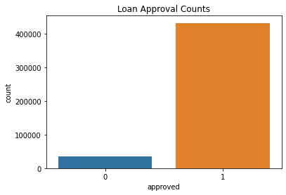
1    431421
0     34864
Name: approved, dtype: int64

After adding the approval feature, we can see that the amount of loan applications classify as approved (1) are higher than the rejected (0). This is an indication that the dataset is imbalanced and we need to:

• Use the proper evaluation metrics such as Precision, Recall, F1, and AUC score to evaluate our model
• Oversampling or Undersampling the data to reduce bias (underfitting) in the minority class

Feature Selection

Since we already have the target label now we need a set of features that I’ll be used as a predictor. In this step, I have done research about the potential features that are usually important for predicting loan applications and consider specific criteria like:

• Features that will only be available in borrower application: some features like loan_status, grade, and funded_amount might not be available, since the borrower is not having a loan yet.
• Features that don’t have too many unique, duplicate, or missing values

The selected features are then stored in the features_selection variable

features_selection=['loan_amnt','dti', 'int_rate', 'emp_length','annual_inc', 'dti', 'delinq_2yrs', 'acc_now_delinq', 'revol_util', 'home_ownership','pymnt_plan', 'purpose', 'addr_state', 'approved']

Encode Categorical Data

There is no single best encoding technique for all datasets, the best encoding technique will depend on the characteristics of your dataset and the specific problem you are trying to solve. However, when dealing with imbalanced datasets and loan prediction problems, there are some encoding techniques that are particularly well-suited:

• The Weight of Evidence (WOE) Encoding: This is a technique for encoding categorical variables that is particularly useful for datasets with imbalanced classes. It works by replacing each category with the log ratio of the probability of the target variable being 1 for that category to the probability of the target variable being 0. This helps to highlight the relationship between each category and the target variable and can be particularly useful for datasets with imbalanced classes.

• Target Encoding: This technique encodes categorical variables by replacing each category with the average value of the target variable for that category. This can help to reduce the number of unique categories and provide more robust feature encoding. Target encoding can be a good choice when dealing with imbalanced datasets because it can help to highlight the relationship between each category and the target variable.

• LeaveOneOut Encoding: This is a technique for encoding categorical variables that is similar to target encoding. It works by replacing each category with the average value of the target variable for all examples in the dataset, except for the one being encoded. This can help to reduce the number of unique categories and provide more robust feature encoding. LeaveOneOut Encoding can be a good choice when dealing with imbalances.

In this phase, I choose Target Encoding.

X = df_fs.loc[:, df_fs.columns][categorical_features]
y = df_fs.approved

te_encoder = ce.TargetEncoder(cols=categorical_features)
te_encoder.fit(X, y)

X_encoded = te_encoder.transform(X).astype('float32')
X_encoded.columns = ['te_'+col for col in X_encoded.columns]

# concat with features selection dataframe
# and drop old categorical data
df_fs_enc = pd.concat([df_fs, X_encoded], axis=1).drop(categorical_features, axis=1)

Dataset Splitting

After encoding the dataset we can separate the dataset into two groups.

data	% of total	Description
training	80	Data used to tune model parameters $w$ and $b$ in training or fitting
validation	20	Data used to tune other model parameters like degree of polynomial, regularization or the architecture of a neural network.

X = df_fs_enc.drop('approved', axis=1)
y = df_fs_enc.approved

X_train, X_cv, y_train, y_cv = train_test_split(X,y,test_size=0.20, random_state=42, stratify=y)

Feature Scaling

The last step before we perform modeling is we need to scale the data. Feature scaling is applied to ensure that all features are on a similar scale, which can be beneficial for many machine learning algorithms and optimization methods. In this step, I use Robust Scaler since it is less prone to outliers.

r_scaler = RobustScaler()

# Fit only to the training data
X_train_scaled = r_scaler.fit_transform(X_train)

dump(r_scaler, open('r_scaler.pkl', 'wb')) # save r_scaler

X_cv_scaled = r_scaler.transform(X_cv)

Modeling

In the modeling step, the rule of thumb is to start simple and use the simplest model as the baseline and gradually improve the model and the dataset. This technique ensures that the process that we are doing is productive towards making a better and the best model.

Baseline: Logistic Regression

model_baseline = LogisticRegression()
model_baseline.fit(X_train_scaled, y_train)
y_pred = model_baseline.predict(X_cv_scaled)
y_predtrain = model_baseline.predict(X_train_scaled)
CM_LR = confusion_matrix(y_cv,y_pred)
CR_LR = classification_report(y_cv,y_pred)
CM_LRtrain = confusion_matrix(y_train,y_predtrain)
CR_LRtrain = classification_report(y_train,y_predtrain)
print("Confusion Matrix Train:\n",CM_LRtrain)
print("Classification Report Train:\n",CR_LRtrain)
print("Confusion Matrix:\n",CM_LR)
print("Classification Report:\n",CR_LR)

Confusion Matrix Train:
 [[   634  25855]
 [  1538 327932]]
Classification Report Train:
               precision    recall  f1-score   support

           0       0.29      0.02      0.04     26489
           1       0.93      1.00      0.96    329470

    accuracy                           0.92    355959
   macro avg       0.61      0.51      0.50    355959
weighted avg       0.88      0.92      0.89    355959

Confusion Matrix:
 [[  209  6413]
 [  374 81994]]
Classification Report:
               precision    recall  f1-score   support

           0       0.36      0.03      0.06      6622
           1       0.93      1.00      0.96     82368

    accuracy                           0.92     88990
   macro avg       0.64      0.51      0.51     88990
weighted avg       0.89      0.92      0.89     88990

Since the class are imbalanced the model struggling to identify the minority class “0”. From here there are two ways we can do to improve the model which is by modifying the model and the data.

• Data:
  • Apply Resampling techniques such as undersampling or oversampling using SMOTE to mitigate the imbalanced data problem
  • Feature Engineering
• Model:
  • Hyperparameter Tuning

Besides that, there is a need to use a specific plotting technique to see how the model performs on the imbalanced dataset. Based on this post we need to use precision-recall curves for plotting as opposed to ROC curves.

When to Use ROC vs. Precision-Recall Curves?

Generally, the use of ROC curves and precision-recall curves are as follows:

• ROC curves should be used when there are roughly equal numbers of observations for each class.
• Precision-Recall curves should be used when there is a moderate to large class imbalance. The reason for this recommendation is that ROC curves present an optimistic picture of the model on datasets with a class imbalance.

However, ROC curves can present an overly optimistic view of an algorithm’s performance if there is a large skew in the class distribution. […] Precision-Recall (PR) curves, often used in Information Retrieval, has been cited as an alternative to ROC curves for tasks with a large skew in the class distribution.

— The Relationship Between Precision-Recall and ROC Curves, 2006.

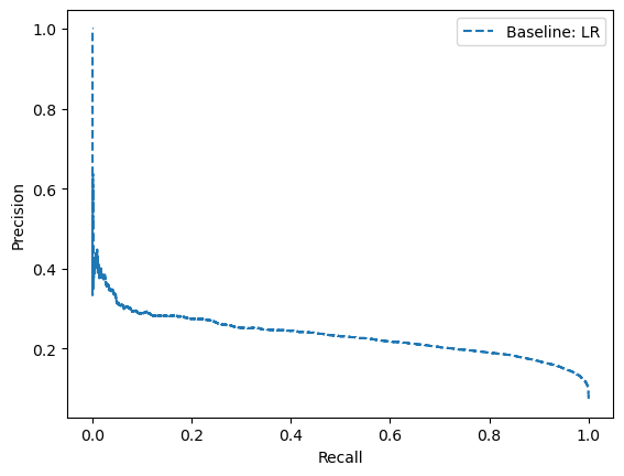
So based on the baseline model I have plotted the model using the Precision-Recall curve using below code.

# predict probabilities
lr_probs = model_baseline.predict_proba(X_cv_scaled)
# keep probabilities for the negative outcome only
lr_probs = lr_probs[:, 0]
# predict class values
yhat = model_baseline.predict(X_cv_scaled)
# calculate precision and recall for each threshold
lr_precision, lr_recall, _ = precision_recall_curve(y_cv, lr_probs, pos_label=0)
# calculate scores
lr_f1, lr_auc = f1_score(y_cv, yhat, pos_label=0), auc(lr_recall, lr_precision)
# summarize scores
print('Logistic: f1=%.3f auc=%.3f' % (lr_f1, lr_auc))
# plot the precision-recall curves
no_skill = len(y_cv[y_cv==0]) / len(y_cv)
#plt.plot([0, 1], [no_skill, no_skill], linestyle='--', label='Baseline')
#plt.plot(lr_recall, lr_precision, marker='.', label='Baseline')
plt.plot(lr_recall, lr_precision, linestyle='--', label='Baseline: LR')
# axis labels
plt.xlabel('Recall')
plt.ylabel('Precision')
# show the legend
plt.legend()
# show the plot
plt.show()

  Logistic: f1=0.058 auc=0.233

Resampling Technique

In this step, we modify the data by applying resampling techniques to mitigate the imbalanced problem. The resampling techniques used in this step are a combination of Oversampling and Undersampling.

Data before resampling

Counter(y_train)

Counter({1: 329470, 0: 26489})

over = SMOTE(sampling_strategy=1)
under = RandomUnderSampler(sampling_strategy=1)
steps = [('o', over), ('u', under)]
pipeline = Pipeline(steps=steps)
X_train_resample, y_train_resample = pipeline.fit_resample(X_train_scaled, y_train)

Data after resampling

Counter(y_train_resample)

Counter({0: 329470, 1: 329470})

We can see after the resampling the proportion of the data is 50/50 for both classes. However, The specific ratio of the minority and majority classes will vary depending on the dataset. To find the best ratio we just have to train the model in different ratios and compare its performances on different ratios.

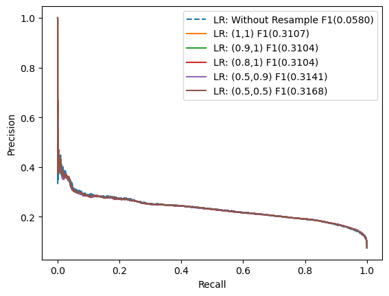
Logistic Regression: Resample ratio Tuning

In this step, I have tried different over and under proportions and see how it affects the performance of the Logistic Regression models.

plot_precision_recall_curve(models_info_resampling_lr)

Random Forest: Resample ratio Tuning

In this step, I have tried different over and under proportions and see how it affects the performance of the Random Forest models.

plot_precision_recall_curve(models_info_resampling_rf)

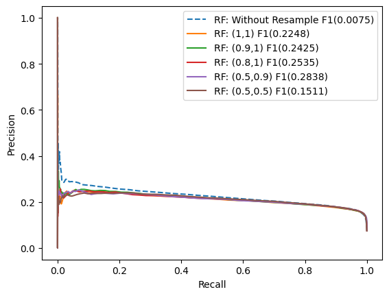
From the above experiment model, we got several findings:

• Resampling does help the model to perform better in classifying minority classes if we compared it with the base model without resampling.
• The portion of under and oversampling slightly affect the F1 score.
• the best portion for sampling_strategy we found really depends on the model, on logistic (0.5, 0,5) is the best, while rf (0.5, 0.9) is the best.
• the (0.5, 0.5) portion is perform worst on rf: resample model, this might indicate that the portion is not stable.

Conclusion: We choose (0.5, 0.9) because it performs well on logistic, and random forest.

Training model with (0.5, 0.9) Resampling data

In this step, I have trained the neural network and XGB model with the new resampled dataset and come up with different F1 scores. In this scenario, logistic Regression produces the highest result for predicting minority class (0), with the second highest neural network.

models_info = pd.concat([models_info, neural_network_data], ignore_index=True)
models_info

	model name	F1-score
1	Logistic Regression	0.3132
2	Neural Network	0.3000
3	Random Forest	0.2872
4	XGBoost	0.2334

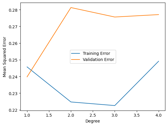
Feature Engineering (Polynomial Degree)

In this step, I’m trying to create new features using polynomial degrees, polynomial degree features will produce a more complex model to capture more complex relationships in our data.

train_errors = []
val_errors = []

# Iterate over polynomial degrees
for degree in range(1, 5):
    # Create polynomial features
    poly = PolynomialFeatures(degree=degree)
    X_poly_train = poly.fit_transform(X_train_resample)
    X_poly_val = poly.transform(X_cv_scaled)
    
     # Create and fit LinearRegression model
    model = LogisticRegression()
    model.fit(X_poly_train, y_train_resample)

    # Predict and calculate mean squared error
    y_train_pred = model.predict(X_poly_train)
    y_val_pred = model.predict(X_poly_val)
    train_mse = mean_squared_error(y_train_resample, y_train_pred)
    val_mse = mean_squared_error(y_cv, y_val_pred)

    train_errors.append((degree, train_mse))
    val_errors.append((degree, val_mse))

What is the good number of polynomial degrees?

When we’re talking about polynomial degrees, it’s a trade-off between the accuracy and complexity of the model. In this case, three offers complexity with a reasonable amount of error.

# Plot training vs validation error
train_errors = np.array(train_errors)
val_errors = np.array(val_errors)

fig, ax = plt.subplots()
ax.plot(train_errors[:,0], train_errors[:,1], label='Training Error')
ax.plot(val_errors[:,0], val_errors[:,1], label='Validation Error')
ax.legend()
ax.set_xlabel('Degree')
ax.set_ylabel('Mean Squared Error')
plt.show()

Hyperparameter tuning

In this step, we will do hyperparameter tuning I will only try hyperparameter tuning on the LR model to make it short since it produces the best F1 score from the previous recap

Logistic Regression

lr_tuning = LogisticRegression(random_state=42)
param_grid = {
        'C': [0.001, 0.01, 0.1, 1, 10, 100],
        'penalty': ['l1', 'l2'],
        'fit_intercept': [True, False],
        'solver': ['newton-cg', 'lbfgs', 'liblinear', 'sag'],
        'max_iter': [100, 200, 500, 1000]}

clf_lr_tuning = RandomizedSearchCV(lr_tuning, param_distributions = param_grid, cv = 5, verbose = True, n_jobs = -1)
best_clf_lr_tuning = clf_lr_tuning.fit(X_poly_train,y_train_resample)

Best Score: 0.7741371667110801
Best Parameters: {'solver': 'liblinear', 'penalty': 'l2', 'max_iter': 1000, 'fit_intercept': True, 'C': 100}
Training Accuracy: 0.7746317281675116
Validation Accuracy: 0.7187886279357231
Confusion Matrix:
 [[ 5415  1207]
 [23818 58550]]
Classification Report:
               precision    recall  f1-score   support

           0       0.19      0.82      0.30      6622
           1       0.98      0.71      0.82     82368

    accuracy                           0.72     88990
   macro avg       0.58      0.76      0.56     88990
weighted avg       0.92      0.72      0.79     88990

F1: tf.Tensor(0.8239226, shape=(), dtype=float32)
Area under precision (AUC) Recall: 0.9641245892153532

From the output, the model produces a 0.82 F1-score and 0.96 AUC score which is good for Loan Application prediction.

Project Report

After completing this project I created the PowerPoint presentation using Google Slides which can be accessed below.

These are just summaries of what I have done if you wanna take a look into more details you can access the full notebook on GitHub here.